
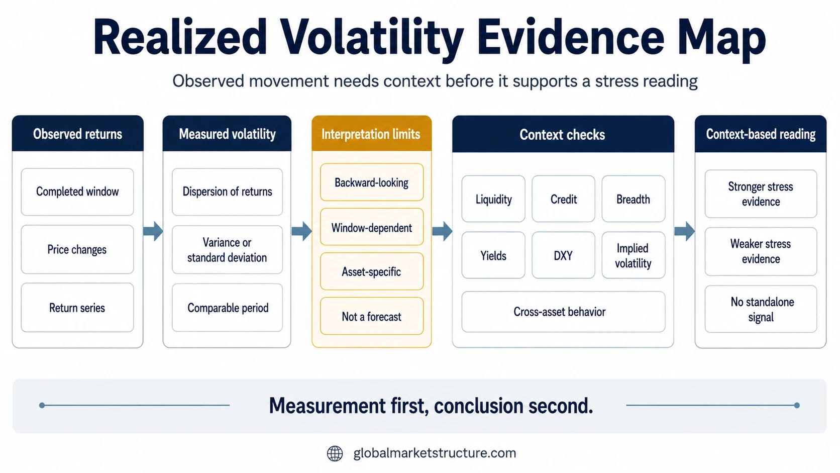
Realized volatility measures price movement that has already occurred over a defined period. It is calculated from observed returns rather than option prices, so the reading is backward-looking. The number depends on how the measurement window, sampling frequency, estimator, and annualization convention are defined.
How Realized Volatility Is Measured
A realized-volatility calculation begins with a return series over a completed period. The exact method varies, but the analytical sequence is consistent: define the observations, measure return variation, and state how the result has been scaled.
A daily close-to-close series and a five-minute intraday series describe the same underlying market through different sets of observations.
The calculation uses changes in price rather than the absolute price level.
The result may be expressed over the original measurement period or annualized for comparison with other volatility measures.
A common close-to-close estimate uses the standard deviation of periodic returns and annualizes it with a factor appropriate to the sampling interval. In high-frequency realized-volatility research, realized variance is commonly constructed by summing squared intraday returns over the evaluation period, with realized volatility derived from that variation measure.
CME educational material describes realized or historical volatility using the standard deviation of past returns and highlights the importance of the observation period and annualization. Federal Reserve research on high-frequency realized volatility aggregates intraday return variation and shows that sampling frequency can affect the estimate when market microstructure noise becomes material. Source: CME Group. Source: Federal Reserve.
Why Two Realized-Volatility Readings Can Differ
A close-to-close volatility estimate and an intraday realized-volatility estimate can both describe observed movement while producing different values. The difference can come from the data frequency and estimator rather than from a disagreement about what the market did.
Uses periodic returns such as daily closes and commonly summarizes their dispersion with standard deviation.
Uses multiple observations inside the evaluation period and can aggregate squared intraday returns into realized variance.
| Measurement choice | What changes | Why it matters |
|---|---|---|
| Window length | The amount of past data included | A short window reacts faster to recent movement, while a longer window incorporates more history. |
| Sampling frequency | How often returns are observed | Daily and intraday observations can capture different parts of the price path. |
| Estimator | How return variation is summarized | Standard deviation, summed squared returns, and more specialized estimators need not produce identical readings. |
| Annualization | How the measured variation is scaled | Comparisons require consistent scaling conventions. |
| Market data quality | How accurately the return series represents tradable prices | Stale prices, illiquidity, and very high sampling frequencies can affect the estimate. |
Realized Volatility and Implied Volatility
Realized volatility describes movement already observed in the return series. Implied volatility is inferred from current option prices and refers to volatility pricing for a future horizon.
Comparing the two requires consistent horizons and clear measurement definitions. The dedicated implied vs realized volatility page covers that relationship in detail.
How Realized Volatility Fits Stress and Regime Analysis
Higher realized volatility establishes that larger movement occurred during the measured period. It does not identify the cause of that movement. Credit conditions, liquidity, breadth, cross-asset behavior, and other evidence determine whether the observed movement belongs to a broader stress interpretation.
Persistence adds a different layer. Repeated elevated or subdued readings can contribute to a volatility regime assessment, but regime classification depends on behavior across multiple observations rather than one completed window.
The reading should remain tied to its window, sampling frequency, estimator, and asset. A high value can document a turbulent period without proving that stress will persist, while a low value can document quiet movement without establishing that the broader market environment is safe.